
Token
Member
First, let me say I am not 100% sure this should be in this forum, possibly it belongs more in Off Topic Wireless, if so I am sure Wayne will hook it up.
Although I am primarily an HF monitor (both for aviation and other things) I do occasionally delve into other bands.
First, a picture:
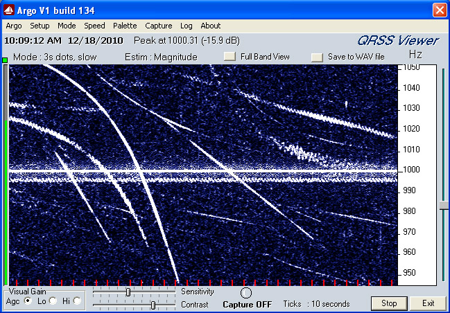
What is going on in this image? Aircraft are in transit, most of them in this image probably to and from LAX or other airfields in the LA Basin. The curves and slopes are aircraft Doppler shifts of the carrier frequency represented by the solid straight line across the center of the image. The carrier is the ATSC carrier from Los Angeles KABC TV Channel 7, on 174.310 MHz.
The ATSC carrier is received on a radio with SSB capability, in this case an Icom R8500 in USB mode (any transmitted carrier at any frequency and from any source can be used, but to work best it should be an unmodulated or steady carrier, or a carrier with the modulation starting at least 1 kHz from the carrier frequency, if not the Doppler shifted signals can be difficult to separate from the modulation). The audio from the receiving radio is put into the sound card of a PC and an audio spectrogram program (in this case Argo 1.34) is used to show a waterfall of the audio spectrum.
As an aircraft flies through the air radio frequencies, from up and down the spectrum, are reflected off of its skin, identical in function to radar. Because the aircraft is generally in motion compared to the transmitter source the reflections are Doppler shifted. The magnitude (in frequency) of the Doppler shift is dependant on two things, the original carrier frequency and the target radial velocity to the transmitter. The higher the carrier frequency the larger the Doppler shift will be for a given radial velocity. The radial velocity is not, necessarily, the same as the true velocity of the aircraft, these two would only be equal if the aircraft was flying directly towards, or away from, the transmitter source.
Now, Argo is very simple to use for this application, but often has a limited bandwidth that can be displayed for useful waterfall scroll speeds and levels of detail. In the above picture example you can only see about + and – 53 Hz, meaning the target radial velocity must be no more than + and – about 90 knots (remember, radial velocity to the transmitter site, not real velocity of the target). And the time from one end to the other is only about 5 minutes 30 seconds of history.
Another example:
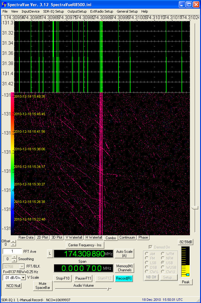
This one is done a little differently, using an SDR-IQ and SpectraVue on the IF output of the Icom R8500 instead of the audio. The advantage here is wider bandwidth and more adaptability of waterfall scroll speeds. This image shows 700 Hz of width and 30 minutes of history. 700 Hz means I can see Doppler shifts of up to + and – 350 Hz, or radial velocities of up to 585 knots. In fact the two tracks in the lower left corner of the picture are at that speed and increasing.
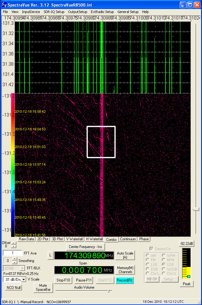
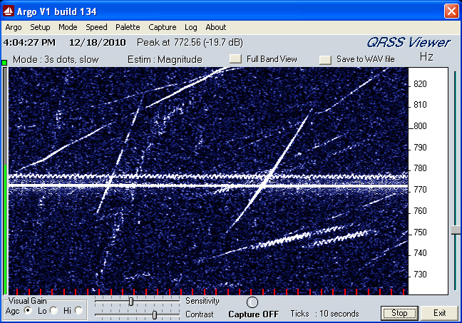
The relative differences can be seen in the following two images, the top one is in SpectraVuethe second in Argo. The white-bordered rectangle in the first image is the coverage area for Argo and you can see the same returns inside it as in the full Argo shot:
Sometimes I have been able to correlate Doppler tracks with aircraft by monitoring LAX. When LAX approach or departure control commands a course correction you can sometimes see the radial velocity track change. The same thing with speed changes, LAX might tell a flight to reduce speed to such-and-such and you can see the curve change with the speed change. And when LAX is turning everyone at the same point you can anticipate such changes for each aircraft, sometimes Iding many aircraft in a row.
Helicopters can sometimes be differentiated from other aircraft because the rotors have a Doppler frequency all their own (think about it, each blade has a separate and constantly changing radial velocity as it goes around and around), and you can see the modulation on the other curve.
I post this thinking that other folks interested in aircraft might like to take a stab at “monitoring” them a different way. I must admit, the use of the ATSC carriers is not my idea, Jon-FL in the #wunclub IRC channel suggested it to me. I have seen this affect before on HF freqs but it is infrequent, few and far between. I am fortunate that the geometry works well for me and the high traffic LA area, I am about 120 air miles from LA. Other areas might not show the level of activity that I see here.
T!
Mohave Desert, California, USA
Although I am primarily an HF monitor (both for aviation and other things) I do occasionally delve into other bands.
First, a picture:
What is going on in this image? Aircraft are in transit, most of them in this image probably to and from LAX or other airfields in the LA Basin. The curves and slopes are aircraft Doppler shifts of the carrier frequency represented by the solid straight line across the center of the image. The carrier is the ATSC carrier from Los Angeles KABC TV Channel 7, on 174.310 MHz.
The ATSC carrier is received on a radio with SSB capability, in this case an Icom R8500 in USB mode (any transmitted carrier at any frequency and from any source can be used, but to work best it should be an unmodulated or steady carrier, or a carrier with the modulation starting at least 1 kHz from the carrier frequency, if not the Doppler shifted signals can be difficult to separate from the modulation). The audio from the receiving radio is put into the sound card of a PC and an audio spectrogram program (in this case Argo 1.34) is used to show a waterfall of the audio spectrum.
As an aircraft flies through the air radio frequencies, from up and down the spectrum, are reflected off of its skin, identical in function to radar. Because the aircraft is generally in motion compared to the transmitter source the reflections are Doppler shifted. The magnitude (in frequency) of the Doppler shift is dependant on two things, the original carrier frequency and the target radial velocity to the transmitter. The higher the carrier frequency the larger the Doppler shift will be for a given radial velocity. The radial velocity is not, necessarily, the same as the true velocity of the aircraft, these two would only be equal if the aircraft was flying directly towards, or away from, the transmitter source.
Now, Argo is very simple to use for this application, but often has a limited bandwidth that can be displayed for useful waterfall scroll speeds and levels of detail. In the above picture example you can only see about + and – 53 Hz, meaning the target radial velocity must be no more than + and – about 90 knots (remember, radial velocity to the transmitter site, not real velocity of the target). And the time from one end to the other is only about 5 minutes 30 seconds of history.
Another example:
This one is done a little differently, using an SDR-IQ and SpectraVue on the IF output of the Icom R8500 instead of the audio. The advantage here is wider bandwidth and more adaptability of waterfall scroll speeds. This image shows 700 Hz of width and 30 minutes of history. 700 Hz means I can see Doppler shifts of up to + and – 350 Hz, or radial velocities of up to 585 knots. In fact the two tracks in the lower left corner of the picture are at that speed and increasing.
The relative differences can be seen in the following two images, the top one is in SpectraVuethe second in Argo. The white-bordered rectangle in the first image is the coverage area for Argo and you can see the same returns inside it as in the full Argo shot:
Sometimes I have been able to correlate Doppler tracks with aircraft by monitoring LAX. When LAX approach or departure control commands a course correction you can sometimes see the radial velocity track change. The same thing with speed changes, LAX might tell a flight to reduce speed to such-and-such and you can see the curve change with the speed change. And when LAX is turning everyone at the same point you can anticipate such changes for each aircraft, sometimes Iding many aircraft in a row.
Helicopters can sometimes be differentiated from other aircraft because the rotors have a Doppler frequency all their own (think about it, each blade has a separate and constantly changing radial velocity as it goes around and around), and you can see the modulation on the other curve.
I post this thinking that other folks interested in aircraft might like to take a stab at “monitoring” them a different way. I must admit, the use of the ATSC carriers is not my idea, Jon-FL in the #wunclub IRC channel suggested it to me. I have seen this affect before on HF freqs but it is infrequent, few and far between. I am fortunate that the geometry works well for me and the high traffic LA area, I am about 120 air miles from LA. Other areas might not show the level of activity that I see here.
T!
Mohave Desert, California, USA

")